Note
Go to the end to download the full example code.
Use the Xtract feature#
This example shows how to use the Xtract feature in PyAnsys Sound. It demonstrates different capabilities of this feature, such as noise extraction, tonal extraction, and transient extraction.
# Maximum frequency for STFT plots, change according to your need
MAX_FREQUENCY_PLOT_STFT = 5000.0
Set up analysis#
Setting up the analysis consists of loading Ansys libraries, connecting to the DPF server, and retrieving the example files.
# Load Ansys libraries.
import os

import matplotlib.pyplot as plt
import numpy as np

from ansys.sound.core.examples_helpers import (
    download_xtract_demo_signal_1_wav,
    download_xtract_demo_signal_2_wav,
)
from ansys.sound.core.server_helpers import connect_to_or_start_server
from ansys.sound.core.signal_utilities import CropSignal, LoadWav
from ansys.sound.core.spectrogram_processing import Stft
from ansys.sound.core.xtract import (
    Xtract,
    XtractDenoiser,
    XtractDenoiserParameters,
    XtractTonal,
    XtractTonalParameters,
    XtractTransient,
    XtractTransientParameters,
)

# Connect to a remote server or start a local server
my_server = connect_to_or_start_server(use_license_context=True)
Define a custom function for STFT plots#
Define a custom function for STFT plots lets you have
more control over what you are displaying.
While you could use the Stft.plot() method, the custom function
defined here restricts the frequency range of the plot.
def plot_stft(stft_class, SPLmax, title="STFT", maximum_frequency=MAX_FREQUENCY_PLOT_STFT):
    """Plot a short-term Fourier transform (STFT) into a figure window.

    Parameters
    ----------
    stft_class: Stft
        Object containing the STFT.
    SPLmax: float
        Maximum value (here in dB SPL) for the colormap.
    title: str
        Title of the figure.
    maximum_frequency: float
        Maximum frequency in Hz to display.
    """
    out = stft_class.get_output_as_nparray()

    # Extract first half of the STFT (second half is symmetrical)
    half_nfft = int(out.shape[0] / 2) + 1
    magnitude = stft_class.get_stft_magnitude_as_nparray()

    # Voluntarily ignore a numpy warning
    np.seterr(divide="ignore")
    magnitude = 20 * np.log10(magnitude[0:half_nfft, :])
    np.seterr(divide="warn")

    # Obtain sampling frequency, time steps, and number of time samples
    fs = 1.0 / (
        stft_class.signal.time_freq_support.time_frequencies.data[1]
        - stft_class.signal.time_freq_support.time_frequencies.data[0]
    )
    time_step = np.floor(stft_class.fft_size * (1.0 - stft_class.window_overlap) + 0.5) / fs
    num_time_index = len(stft_class.get_output().get_available_ids_for_label("time"))

    # Define boundaries of the plot
    extent = [0, time_step * num_time_index, 0.0, fs / 2.0]

    # Plot
    plt.figure()
    plt.imshow(
        magnitude,
        origin="lower",
        aspect="auto",
        cmap="jet",
        extent=extent,
        vmax=SPLmax,
        vmin=(SPLmax - 70.0),
    )
    plt.colorbar(label="Magnitude (dB SPL)")
    plt.ylabel("Frequency (Hz)")
    plt.xlabel("Time (s)")
    plt.ylim([0.0, maximum_frequency])  # Change the value of MAX_FREQUENCY_PLOT_STFT if needed
    plt.title(title)
    plt.show()
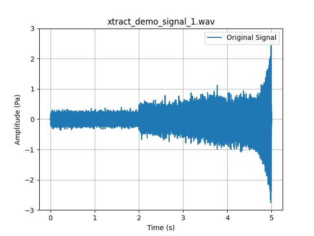
Load a demo signal for Xtract#
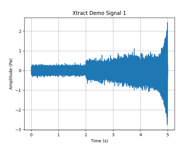
Load a demo signal from a WAV file using the LoadWav class.
The WAV file contains harmonics and shocks.
# Return the input data of the example file
path_xtract_demo_signal_1 = download_xtract_demo_signal_1_wav()
# Load the WAV file
wav_loader = LoadWav(path_to_wav=path_xtract_demo_signal_1)
wav_loader.process()
# Plot the signal in time domain
time_domain_signal = wav_loader.get_output()[0]
time_vector = time_domain_signal.time_freq_support.time_frequencies.data
plt.plot(time_vector, time_domain_signal.data)
plt.title("Xtract Demo Signal 1")
plt.grid(True)
plt.xlabel("Time (s)")
plt.ylabel("Amplitude (Pa)")
plt.show()
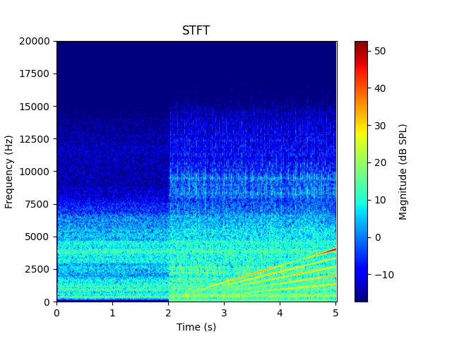
# Compute the spectrogram of the signal and plot it
stft_original = Stft(signal=wav_loader.get_output()[0], fft_size=1024, window_overlap=0.9)
stft_original.process()
max_stft = 20 * np.log10(np.max(stft_original.get_stft_magnitude_as_nparray()))
plot_stft(stft_original, SPLmax=max_stft, maximum_frequency=20000.0)
Use individual extraction features#
The following topics show how to use different capabilities of Xtract independently.
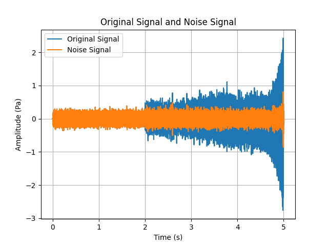
Noise extraction#
The goal is to isolate a fan noise deprived of any tonal content in the demo signal.
# Create a noise pattern using the first two seconds of the signal.
# First crop the first two seconds of the signal.
signal_cropper = CropSignal(signal=time_domain_signal, start_time=0.0, end_time=2.0)
signal_cropper.process()
cropped_signal = signal_cropper.get_output()

# Then use the 'XtractDenoiserParameters' class to create the noise pattern.
xtract_denoiser_params = XtractDenoiserParameters()
xtract_denoiser_params.noise_psd = xtract_denoiser_params.create_noise_psd_from_noise_samples(
    signal=cropped_signal, sampling_frequency=44100.0, window_length=100
)

# Denoise the signal using the 'XtractDenoiser' class.
xtract_denoiser = XtractDenoiser(
    input_signal=time_domain_signal, input_parameters=xtract_denoiser_params
)
xtract_denoiser.process()

noise_signal = xtract_denoiser.get_output()[1]

# Plot the original signal and the noise signal in the same window
plt.plot(time_vector, time_domain_signal.data, label="Original Signal")
plt.plot(time_vector, noise_signal.data, label="Noise Signal")
plt.grid(True)
plt.xlabel("Time (s)")
plt.ylabel("Amplitude (Pa)")
plt.title("Original Signal and Noise Signal")
plt.legend()
plt.show()
Tone extraction#
The goal is to isolate the tones using the right settings.
# Try a first attempt of tone extraction with a
# First set of parameters using the 'XtractTonalParameters' class.
xtract_tonal_params = XtractTonalParameters()
xtract_tonal_params.regularity = 1.0
xtract_tonal_params.maximum_slope = 1000.0
xtract_tonal_params.minimum_duration = 0.22
xtract_tonal_params.intertonal_gap = 10.0
xtract_tonal_params.local_emergence = 2.0
xtract_tonal_params.fft_size = 2048

## Now perform the tonal extraction using the 'XtractTonal' class
xtract_tonal = XtractTonal(input_signal=time_domain_signal, input_parameters=xtract_tonal_params)
xtract_tonal.process()
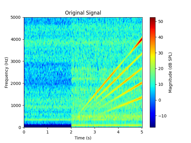
Plot the spectrogram to assess the quality of the output.
stft_modified_signal = Stft(signal=xtract_tonal.get_output()[0], fft_size=1024, window_overlap=0.9)
stft_modified_signal.process()
print("Plot of the spectrograms with tonal extraction parameters that do not work.")
## Spectrogram of the original signal
plot_stft(stft_original, SPLmax=max_stft, title="Original Signal")
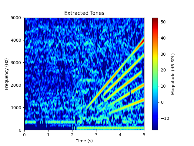
## Spectrogram of the modified signal
plot_stft(stft_modified_signal, SPLmax=max_stft, title="Extracted Tones")
# You can see from the obtained plot that the tones are not properly extracted.

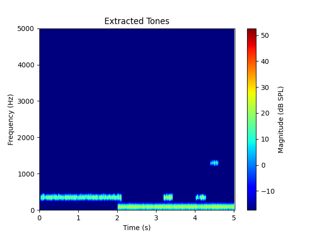
Plot of the spectrograms with tonal extraction parameters that do not work.
Try again with a different parameter for the maximum slope.
xtract_tonal_params.maximum_slope = 5000.0
xtract_tonal.process()

# Recheck the plots
print("Plot of the spectrograms with the right tonal extraction parameters.")
plot_stft(stft_original, SPLmax=max_stft, title="Original Signal")

# Spectrogram of the modified signal
stft_modified_signal.signal = xtract_tonal.get_output()[0]
stft_modified_signal.process()
plot_stft(stft_modified_signal, SPLmax=max_stft, title="Extracted Tones")
Plot of the spectrograms with the right tonal extraction parameters.
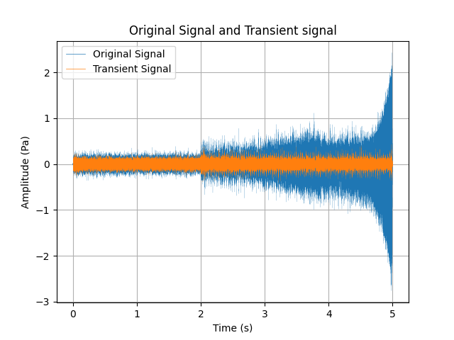
Transient extraction#
The goal is to isolate the transients using the right settings. While these settings are not as easy to handle, they are well explained in the tutorial videos installed with the Ansys Sound Analysis and Specification (SAS) standalone application (with the user interface). You can also find the SAS - XTRACT transient videos on the Ansys Learning Hub.
# Create a set of transient parameters.
# This example assumes that the best minimum and maximum thresholds are known.
# You can use the SAS interface to help set up these thresholds interactively.
xtract_transient_params = XtractTransientParameters(lower_threshold=51.5, upper_threshold=60.0)

# Perform the transient extraction using the 'XtractTransient' class.
xtract_transient = XtractTransient(
    input_signal=time_domain_signal, input_parameters=xtract_transient_params
)
xtract_transient.process()
transient_signal = xtract_transient.get_output()[0]

# Plot the original signal and the transient signal in the same window
plt.plot(time_vector, time_domain_signal.data, label="Original Signal", linewidth=0.1)
plt.plot(time_vector, transient_signal.data, label="Transient Signal", linewidth=0.1)
plt.grid(True)
plt.xlabel("Time (s)")
plt.ylabel("Amplitude (Pa)")
plt.title("Original Signal and Transient signal")
leg = plt.legend()
for line in leg.get_lines():
    line.set_linewidth(0.5)
plt.show()
Use a combination of extraction features and loop on several signals#
The idea here is to loop over several signals and use the Xtract class to combine
all previous classes.
path_xtract_demo_signal_2 = download_xtract_demo_signal_2_wav()
paths = [path_xtract_demo_signal_1, path_xtract_demo_signal_2]
# Instantiate the 'Xtract' class with the parameters previously set
xtract = Xtract(
parameters_denoiser=xtract_denoiser_params,
parameters_tonal=xtract_tonal_params,
parameters_transient=xtract_transient_params,
)
# Loop over all signal paths contained in the 'paths' variable
for p in paths:
# Name the signal using the file name
signal_name = os.path.basename(p)
# Load the signal
wav_loader.path_to_wav = p
wav_loader.process()
time_domain_signal = wav_loader.get_output()[0]
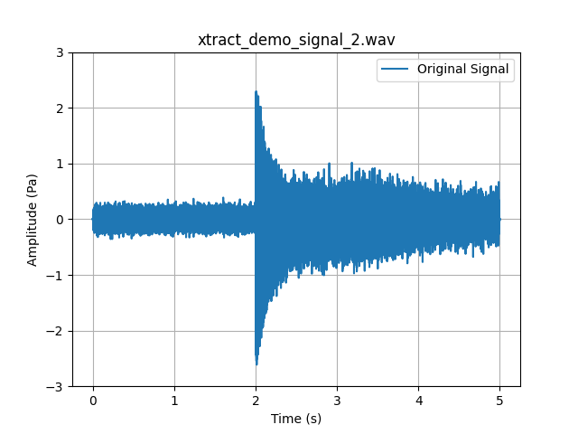
# Plot the time domain signal
ylims = [-3.0, 3.0]
plt.figure()
plt.plot(time_vector, time_domain_signal.data, label="Original Signal")
plt.ylim(ylims)
plt.ylabel("Amplitude (Pa)")
plt.xlabel("Time (s)")
plt.grid()
plt.legend()
plt.title(signal_name)
plt.show()
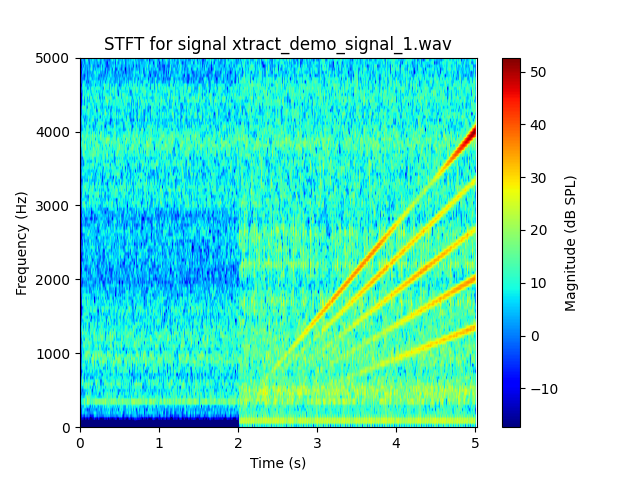
# Compute and plot the STFT
stft_original.signal = time_domain_signal
stft_original.process()
plot_stft(stft_class=stft_original, SPLmax=max_stft, title=f"STFT for signal {signal_name}")
# Use Xtract with the loaded signal
xtract.input_signal = time_domain_signal
xtract.process()
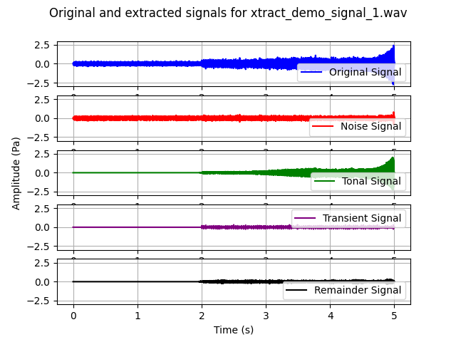
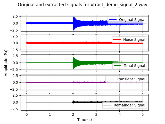
# Collect outputs and plot everything in one window
noise_signal, tonal_signal, transient_signal, remainder_signal = xtract.get_output()
f, axs = plt.subplots(nrows=5)
axs[0].plot(time_vector, time_domain_signal.data, label="Original Signal", color="blue")
axs[1].plot(time_vector, noise_signal.data, label="Noise Signal", color="red")
axs[2].plot(time_vector, tonal_signal.data, label="Tonal Signal", color="green")
axs[2].set(ylabel="Amplitude (Pa)") # Set ylabel for middle plot only
axs[3].plot(time_vector, transient_signal.data, label="Transient Signal", color="purple")
axs[4].plot(time_vector, remainder_signal.data, label="Remainder Signal", color="black")
for ax in axs:
ax.set_ylim(ylims)
ax.grid()
ax.legend()
ax.set_aspect("auto")
plt.xlabel("Time (s)")
plt.legend()
plt.suptitle(f"Original and extracted signals for {signal_name}")
plt.show()

Total running time of the script: (12 minutes 43.565 seconds)