Load a signal from a WAV file

This example shows how to load a signal from a WAV file, modify the signal’s sampling frequency, and amplify it. It also shows how to access the corresponding data, display it using Matplotlib, and then write the modified signal to the disk as a new WAV file.

Set up analysis

Setting up the analysis consists of loading Ansys libraries, connecting to the DPF server, and retrieving the example files.

# Load Ansys and other libraries.
import matplotlib.pyplot as plt

from ansys.sound.core.examples_helpers import download_flute_wav
from ansys.sound.core.server_helpers import connect_to_or_start_server
from ansys.sound.core.signal_utilities import ApplyGain, LoadWav, Resample, WriteWav

# Connect to a remote server or start a local server
server = connect_to_or_start_server()

Load a signal

Load a signal from a WAV file using the LoadWav class. It is returned as a DPF fields container. For more information, see fields_container in the DPF-Core API documentation.

# Return the input data of the example file
path_flute_wav = download_flute_wav()

# Load the WAV file.
wav_loader = LoadWav(path_flute_wav)
wav_loader.process()
fc_signal_original = wav_loader.get_output()

t1 = fc_signal_original[0].time_freq_support.time_frequencies.data
sf1 = 1.0 / (t1[1] - t1[0])
print(f"The sampling frequency of the original signal is {int(sf1)} Hz.")

The sampling frequency of the original signal is 44100 Hz.

Resample the signal

Change the sampling frequency of the loaded signal.

resampler = Resample(fc_signal_original, new_sampling_frequency=20000.0)
resampler.process()
fc_signal_resampled = resampler.get_output()

t2 = fc_signal_resampled[0].time_freq_support.time_frequencies.data
sf2 = 1.0 / (t2[1] - t2[0])
print(f"The new sampling frequency of the signal is {int(sf2)} Hz.")

The new sampling frequency of the signal is 20000 Hz.

Apply a gain to the signal

Amplify the resampled signal by 10 decibels.

gain = 10.0
gain_applier = ApplyGain(fc_signal_resampled, gain=gain, gain_in_db=True)
gain_applier.process()
fc_signal_modified = gain_applier.get_output()

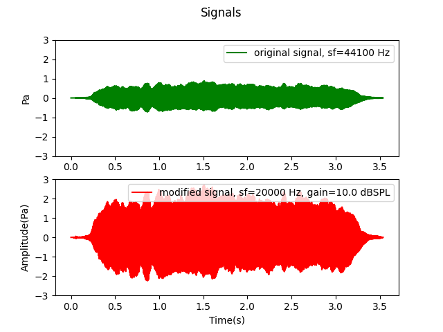
Plot signals

Plot both the original signal and modified signal.

# Get the signals as nparray
data_original = wav_loader.get_output_as_nparray()
data_modified = gain_applier.get_output_as_nparray()

# Prepare the figure
fig, axs = plt.subplots(2)
fig.suptitle("Signals")

axs[0].plot(t1, data_original, color="g", label=f"original signal, sf={int(sf1)} Hz")
axs[0].set_ylabel("Pa")
axs[0].legend(loc="upper right")
axs[0].set_ylim([-3, 3])

axs[1].plot(
    t2, data_modified, color="r", label=f"modified signal, sf={int(sf2)} Hz, gain={gain} dBSPL"
)
axs[1].set_xlabel("Time(s)")
axs[1].set_ylabel("Amplitude(Pa)")
axs[1].legend(loc="upper right")
axs[1].set_ylim([-3, 3])

# Display the figure
plt.show()

Write the signal as a WAV file

Write the modified signal to the disk as a WAV file.

output_path = path_flute_wav[:-4] + "_modified.wav"  # "[-4]" is to remove the ".wav" extension
wav_writer = WriteWav(path_to_write=output_path, signal=fc_signal_modified, bit_depth="int16")
wav_writer.process()