Isolate orders

Orders are harmonic and partial components in the sound related to the speed of a rotating machine. This example shows how to isolate orders in a signal containing an RPM profile. It also uses additional classes from PyAnsys Sound to compute spectrograms and the loudness of the isolated signals.

# Maximum frequency for STFT plots, change according to your need
MAX_FREQUENCY_PLOT_STFT = 2000.0

Set up analysis

Setting up the analysis consists of loading the required libraries, connecting to the DPF server, and retrieving the example files.

# Load standard libraries.
import matplotlib.pyplot as plt
import numpy as np

# Load Ansys libraries.
from ansys.sound.core.examples_helpers import (
    download_accel_with_rpm_2_wav,
    download_accel_with_rpm_3_wav,
    download_accel_with_rpm_wav,
)
from ansys.sound.core.psychoacoustics import LoudnessISO532_1_Stationary
from ansys.sound.core.server_helpers import connect_to_or_start_server
from ansys.sound.core.signal_utilities import LoadWav, WriteWav
from ansys.sound.core.spectrogram_processing import IsolateOrders, Stft


# Connect to a remote DPF server or start a local DPF server.
my_server, my_license_context = connect_to_or_start_server(use_license_context=True)

Define custom STFT plot function

Define a custom function for STFT plots. It differs from the Stft.plot() method in that it does not display the phase and allows setting custom title, maximum SPL, and maximum frequency.

def plot_stft(
    stft: Stft,
    fs: float,
    SPLmax: float,
    title: str = "STFT",
    maximum_frequency: float = MAX_FREQUENCY_PLOT_STFT,
) -> None:
    """Plot a short-term Fourier transform (STFT) into a figure window.

    Parameters
    ----------
    stft: Stft
        Object containing the STFT.
    fs: float
        Sampling frequency of the signal in Hz.
    SPLmax: float
        Maximum value (here in dB SPL) for the colormap.
    title: str, default: "STFT"
        Title of the figure.
    maximum_frequency: float, default: MAX_FREQUENCY_PLOT_STFT
        Maximum frequency in Hz to display.
    """
    magnitude = stft.get_stft_magnitude_as_nparray()
    magnitude_unit = stft.get_output()[0].unit
    frequency_unit = stft.get_output()[0].time_freq_support.time_frequencies.unit
    time_unit = stft.get_output().time_freq_support.time_frequencies.unit

    # Only extract the first half of the STFT, as it is symmetrical
    half_nfft = int(magnitude.shape[0] / 2) + 1

    # Voluntarily ignore a numpy warning
    np.seterr(divide="ignore")
    magnitude = 20 * np.log10(magnitude[0:half_nfft, :])
    np.seterr(divide="warn")

    # Obtain sampling frequency, time steps, and number of time samples
    time_data_spectrogram = stft.get_output().time_freq_support.time_frequencies.data

    # Define boundaries of the plot
    extent = [time_data_spectrogram[0], time_data_spectrogram[-1], 0.0, fs / 2.0]

    # Plot
    plt.figure()
    plt.imshow(
        magnitude,
        origin="lower",
        aspect="auto",
        cmap="jet",
        extent=extent,
        vmax=SPLmax,
        vmin=SPLmax - 70.0,
    )
    plt.colorbar(label=f"Magnitude ({magnitude_unit})")
    plt.ylabel(f"Frequency ({frequency_unit})")
    plt.xlabel(f"Time ({time_unit})")
    plt.ylim([0.0, maximum_frequency])  # Change the value of MAX_FREQUENCY_PLOT_STFT if needed.
    plt.title(title)
    plt.show()

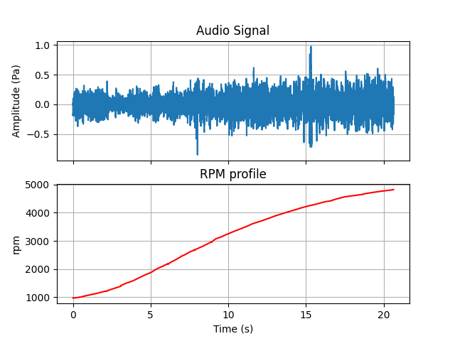
Load a signal with an RPM profile

Load a signal that has been generated with Ansys Sound Analysis and Specification (SAS) from a WAV file using the LoadWav class. This class contains two channels:

• The actual signal (an acceleration recording)

• The associated RPM profile

# Return the input data of the example file.
path_accel_wav = download_accel_with_rpm_wav(server=my_server)

# Load the WAV file.
wav_loader = LoadWav(path_accel_wav)
wav_loader.process()

# Extract the audio signal and the RPM profile.
signal, rpm_profile = wav_loader.get_output()
fs = wav_loader.get_sampling_frequency()

# Extract time support associated with the signal.
time = signal.time_freq_support.time_frequencies

# Plot the signal and its associated RPM profile.
fig, ax = plt.subplots(nrows=2, sharex=True)
ax[0].plot(time.data, signal.data)
ax[0].set_title("Audio Signal")
ax[0].set_ylabel(f"Amplitude ({signal.unit})")
ax[0].grid(True)
ax[1].plot(time.data, rpm_profile.data, color="red")
ax[1].set_title("RPM profile")
ax[1].set_ylabel(f"RPM")
ax[1].grid(True)
plt.xlabel(f"Time ({time.unit})")
plt.show()

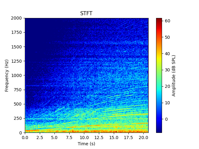
Plot spectrogram of the original signal

Plot the spectrogram of the original signal.

stft = Stft(signal=signal, window_overlap=0.9, fft_size=8192)
stft.process()
max_stft = 20 * np.log10(np.max(stft.get_stft_magnitude_as_nparray()))
plot_stft(stft, fs, max_stft)

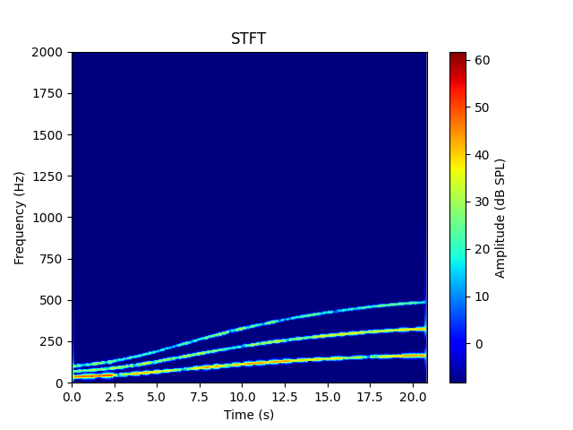
Isolate orders

Isolate orders 2, 4, and 6 with the IsolateOrders class.

rpm_profile = wav_loader.get_output()[1]

# Define parameters for order isolation
order_to_isolate = [2, 4, 6]  # Orders indexes to isolate as a list
fft_size = 8192  # FFT Size (in samples)
window_type = "HANN"  # Window type
window_overlap = 0.9  # Window overlap
width_selection = 3  # Width of the order selection in Hz

# Instantiate the ``IsolateOrders`` class with the parameters.
isolate_orders = IsolateOrders(
    signal=signal,
    rpm_profile=rpm_profile,
    orders=order_to_isolate,
    fft_size=fft_size,
    window_type=window_type,
    window_overlap=window_overlap,
    width_selection=width_selection,
)

# Isolate orders.
isolate_orders.process()

# Plot the spectrogram of the isolated orders.
stft.signal = isolate_orders.get_output()
stft.process()
plot_stft(stft, fs, max_stft)

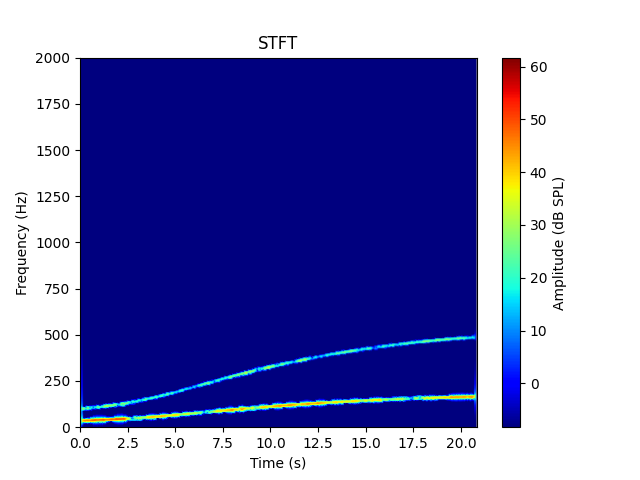
Isolate different orders

Change FFT size, order indexes, and window type. Then re-isolate the orders.

# Change some parameters directly using the setters of the class.
isolate_orders.orders = [2, 6]
isolate_orders.window_type = "BLACKMAN"

# Reprocess (Must be called explicitly. Otherwise, the output won't be updated).
isolate_orders.process()

# Plot the spectrogram of the isolated orders.
stft.signal = isolate_orders.get_output()
stft.process()
plot_stft(stft, fs, max_stft)

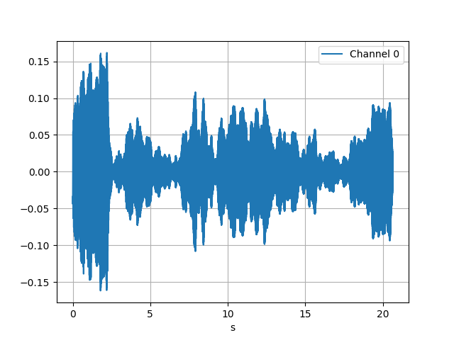
Work with the isolated signal

Plot the signal containing the isolated orders and compute its loudness.

# Plot the signal directly using the method from the ``IsolateOrders`` class.
isolate_orders.plot()

# Use the ``Loudness`` class to compute the loudness of the isolate signal.
signal_isolated = isolate_orders.get_output()
signal_isolated.unit = "Pa"
loudness = LoudnessISO532_1_Stationary(signal=signal_isolated)
loudness.process()

loudness_level_isolated_signal = loudness.get_loudness_level_phon()

# Compute the loudness for the original signal.
loudness.signal = signal
loudness.process()

loudness_level_original_signal = loudness.get_loudness_level_phon()

print(f"The loudness level of the original signal is {loudness_level_original_signal:.1f} phons.")
print(f"The loudness level of the isolated signal is {loudness_level_isolated_signal:.1f} phons.")

The loudness level of the original signal is 76.6 phons.
The loudness level of the isolated signal is 61.4 phons.

Isolate orders of several signals in a loop

Loop over a list of given signals and write them as a WAV file.

path_accel_wav_2 = download_accel_with_rpm_2_wav(server=my_server)
path_accel_wav_3 = download_accel_with_rpm_3_wav(server=my_server)
paths = (path_accel_wav, path_accel_wav_2, path_accel_wav_3)

fft_sizes = [256, 2048, 4096]

wav_writer = WriteWav()

# Isolate orders for all the files containing RPM profiles in this folder.
for file, fft_sz in zip(paths, fft_sizes):
    # Load the file.
    wav_loader.path_to_wav = file
    wav_loader.process()

    # Set parameters for order isolation.
    isolate_orders.signal = wav_loader.get_output()[0]
    isolate_orders.rpm_profile = wav_loader.get_output()[1]
    isolate_orders.fft_size = fft_sz
    isolate_orders.process()

    # Write as a WAV file.
    path_to_write = file[:-4] + "_isolated_fft_size_" + str(fft_sz) + ".wav"
    wav_writer.path_to_write = str(path_to_write)
    wav_writer.signal = isolate_orders.get_output()
    wav_writer.process()