Use an existing Sound Composer project file

The Sound Composer is a tool that allows you to generate the sound of a system by combining the sounds of its components, which we call sources here. Each source can be made of data coming from test analysis, or from a simulation, or simply consist of a single audio recording. The sources are combined into a project, where each source is assigned a track.

A track is a data structure made of source data, source control data, an output gain, and, optionally, a transfer function in the form of a digital filter. It can generate the sound of the component (as characterized by the source data), in specific operating conditions (the source control), and filtered according to the transfer function.

This example shows how to use the Sound Composer, with the SoundComposer class. It starts from an existing Sound Composer project file, and illustrates the notions of project, track, source, source control, and filter.

The example shows how to perform these operations:

• Load a project file,

• Get the project information and content,

• Investigate the content of a track,

• Generate the signal of a track,

• Generate the signal of the entire Sound Composer project.

Set up analysis

Setting up the analysis consists of loading the required libraries, and connecting to the DPF server.

# Load Ansys libraries.
from ansys.sound.core.examples_helpers import download_sound_composer_project_whatif
from ansys.sound.core.server_helpers import connect_to_or_start_server
from ansys.sound.core.sound_composer import SoundComposer
from ansys.sound.core.spectrogram_processing import Stft


# Connect to a remote server or start a local server.
my_server = connect_to_or_start_server(use_license_context=True)

Load a Sound Composer project from a file

Load a Sound Composer project, using the SoundComposer.load() method. A Sound Composer project file has the extension .scn, and can be created with Ansys Sound SAS.

# Download the Sound Composer project file used in this example.
path_sound_composer_project_scn = download_sound_composer_project_whatif(server=my_server)

# Create a SoundComposer object and load the project.
sound_composer_project = SoundComposer()
sound_composer_project.load(path_sound_composer_project_scn)

You can use built-in print() function to display a summary of the content of the project.

print(sound_composer_project)

Sound Composer object (4 track(s))
        Track 1: SourceHarmonics, "eMotor - FEM", gain = +0.0 dB
        Track 2: SourceHarmonics, "Gear - MBD", gain = +0.0 dB
        Track 3: SourceBroadbandNoise, "HVAC - CFD", gain = +0.0 dB
        Track 4: SourceBroadbandNoise, "Road and wind", gain = +0.0 dB

You can see that this project is made of 4 tracks:

• a track with a harmonics source, coming form the FEM simulation of an e-motor,

• a track with another harmonics source, coming from the multibody simulation of a gearbox,

• a track with a broadband noise source, coming from the CFD simulation of a HVAC system,

• a track with another broadband noise source, coming form the analysis of a background noise measurement in the cabin, which would correspond to the rolling noise and the wind noise.

Explore the project’s list of tracks

Let us have a closer look at the content of each individual track by printing it.

for i, track in enumerate(sound_composer_project.tracks, start=1):
    print(f"--- Track n. {i} ---\n {track}\n")

--- Track n. 1 ---
 eMotor - FEM
        Source:
Harmonics source: ''
        Number of orders: 24
                [ 2.  4.  6.  8. 10. ... 40. 42. 44. 46. 48.]
        Control parameter: RPM, 500.0 - 10000.0 rpm
                [ 500. 1000. 2000. 3000. 4000. ...  6000.  7000.  8000.  9000. 10000.]
Source control: RPM
        Min: 250.0
        Max: 5000.0
        Duration: 8.00000037997961 s
        Filter: Set

--- Track n. 2 ---
 Gear - MBD
        Source:
Harmonics source: ''
        Number of orders: 50
                [1. 2. 3. 4. 5. ... 46. 47. 48. 49. 50.]
        Control parameter: RPM, 0.0 - 4960.0 rpm
                [ 0. 20. 40. 60. 80. ... 4880. 4900. 4920. 4940. 4960.]
Source control: RPM
        Min: 250.0
        Max: 5000.0
        Duration: 8.00000037997961 s
        Filter: Set

--- Track n. 3 ---
 HVAC - CFD
        Source:
Broadband noise source: ''
        Spectrum type: Narrow band (DeltaF: 12.2 Hz)
        Spectrum count: 2
        Control parameter: Speed profile_original, rpm
                [2065. 2950.]
Source control: Speed profile_original
        Min: 2600.0
        Max: 2600.0
        Duration: 8.00000037997961 s
        Filter: Not set

--- Track n. 4 ---
 Road and wind
        Source:
Broadband noise source: ''
        Spectrum type: Narrow band (DeltaF: 10.0 Hz)
        Spectrum count: 100
        Control parameter: Speed profile - 2, kph
                [0. 1. 2. 3. 4. ... 95. 96. 97. 98. 99.]
Source control: Speed profile - 2
        Min: 10.0
        Max: 100.0
        Duration: 8.00000037997961 s
        Filter: Not set

For each track, you can see some details about the source content, the associated control profile, and whether the track includes a filter or not.

Explore the content of a track

To look at a specific track, use the attribute tracks of the SoundComposer object, containing the list of the tracks included. For example, let us extract the second track of the project, which contains the gearbox source.

The track object returned is of type Track. You can print it to display its content, as shown in the previous section.

track_gear = sound_composer_project.tracks[1]

This track contains a harmonics source, stored in its Track.source attribute of type SourceHarmonics. Here, it consists of a set of 50 harmonics, which are defined by their order numbers, and their levels over 249 values of the control parameter (RPM).

These data are stored in the SourceHarmonics.source_harmonics attribute of the track’s source object, as a FieldsContainer object. It contains 249 fields, each corresponding to a specific value of the control parameter (RPM), and containing the levels in Pa² of the 50 harmonics at this RPM value.

print(
    f"Number of RPM points defined in the source dataset: "
    f"{len(track_gear.source.source_harmonics)}"
)

Number of RPM points defined in the source dataset: 249

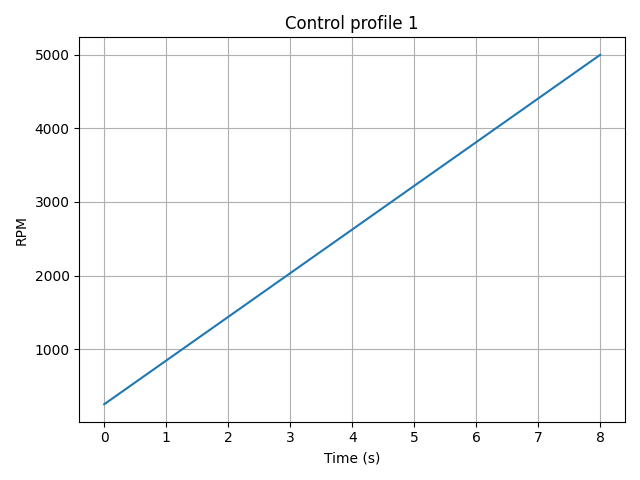
The source control data (that is, the RPM values over time) can be accessed using the SourceHarmonics.source_control attribute of the source in the track. Let us display this control profile in a figure: it is a linear ramp-up from 250 rpm to 5000 rpm, over 8 seconds.

track_gear.source.plot_control()

The track also contains a filter, stored as a Filter object. Here, it is a finite impulse response (FIR) filter that models the transfer between the source and the listening position.

track_gear.filter
print(track_gear.filter)

Sampling frequency: 44100.0 Hz
Numerator coefficients (B): [0.007285992614924908, 0.018362130969762802, 0.02472005784511566, 0.028517061844468117, 0.033101242035627365, ... ]
Denominator coefficients (A): [1.0]

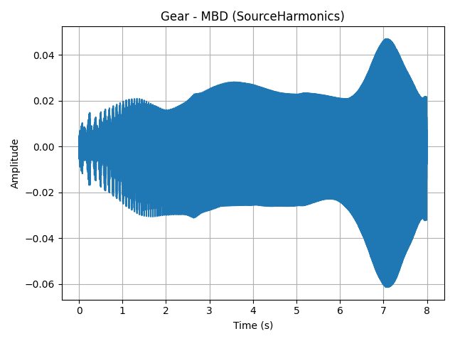
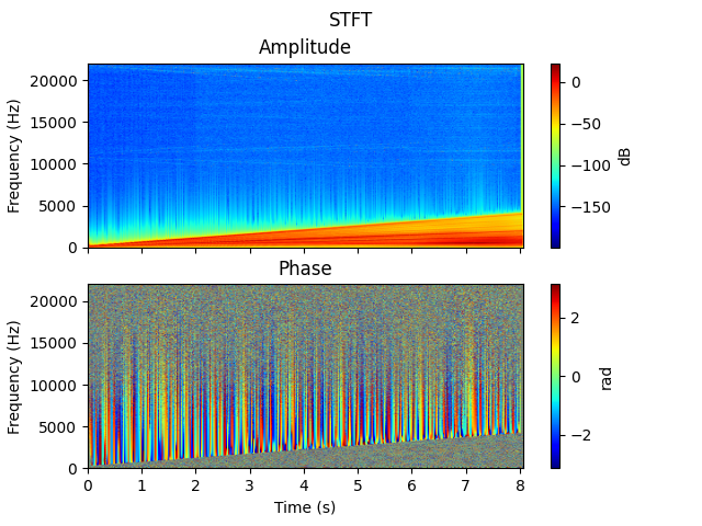
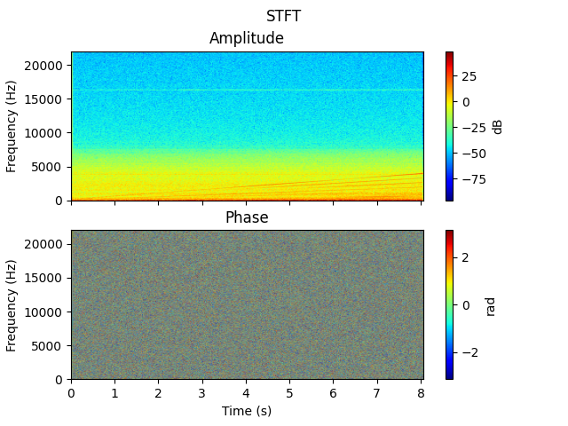
Let us generate the signal corresponding to the track using the Track.process() method, plot its waveform, and display its spectrogram with the Stft class.

track_gear.process(sampling_frequency=44100.0)
track_gear.plot()

spectrogram_gear = Stft(signal=track_gear.get_output())
spectrogram_gear.process()
spectrogram_gear.plot()

• 
• 

If needed, you can access the output signal of a track using Track.get_output().

signal_gear = track_gear.get_output()

Generate the signal of the project

Now, let us generate the signal of the project using the SoundComposer.process() method. This method generates all track signals, filters them with the associated filters whenever specified, applies track gains, and sums the resulting signals together.

sound_composer_project.process(sampling_frequency=44100.0)

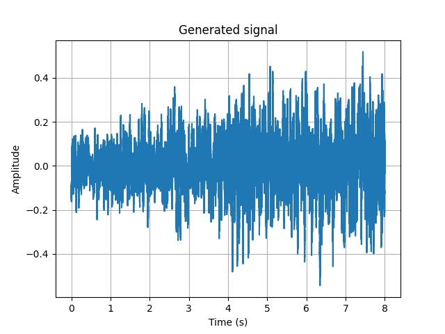
You can display the waveform of the generated signal using the SoundComposer.plot() method, and its spectrogram using the Stft class.

sound_composer_project.plot()

spectrogram = Stft(signal=sound_composer_project.get_output())
spectrogram.process()
spectrogram.plot()

• 
• 

This workflow allows you to analyze and listen to the sound of the gearbox and the e-motor, in realistic conditions, that is, including the HVAC noise and the background noise inside the cabin.

By analyzing the spectrogram, you can anticipate how some harmonic tones from the e-motor and the gearbox may be perceived by the passengers in the cabin.

Further investigations can be conducted, using other tools included in PyAnsys Sound, such as modules Standard levels, Psychoacoustics and Spectral processing.