Calculate RMS, dBSPL and dBA levels

This example shows how to calculate RMS, dBSPL and dBA levels. The following levels are included:

• Overall RMS level

• Overall dBSPL level

• Overall dBA level

• RMS level over time

• dBSPL level over time

• dBA level over time

The example shows how to perform these operations:

• Set up the analysis.

• Calculate levels on loaded WAV files.

• Get calculation outputs.

• Plot some corresponding curves.

• Export levels into a .csv files.

Set up analysis

Setting up the analysis consists of loading Ansys libraries, and connecting to the DPF server.

# Load standard libraries.
import csv
import os

import matplotlib.pyplot as plt

# Load Ansys libraries.
from ansys.sound.core.examples_helpers import (
    download_aircraft_wav,
    download_fan_wav,
)
from ansys.sound.core.server_helpers import connect_to_or_start_server
from ansys.sound.core.signal_utilities import LoadWav
from ansys.sound.core.standard_levels import LevelOverTime, OverallLevel

# Connect to a remote server or start a local server.
my_server = connect_to_or_start_server(use_license_context=True)

Calculate overall RMS, dBSPL and dBA levels

Load a signal from a WAV file using the LoadWav class. It is returned as a FieldsContainer object.

# Load example data from two wav files.
path_fan_wav = download_fan_wav(server=my_server)
path_aircraft_wav = download_aircraft_wav(server=my_server)

Create a first .csv file in which the overall levels will be written, and write the header row.

filepath_overall_results = open("Overall_Results.csv", "w+", newline="")
csv_writer_overall_results = csv.writer(filepath_overall_results)
header_row = ["Signal name", "Overall level [RMS]", "Overall level [dBSPL]", "Overall level [dBA]"]
_ = csv_writer_overall_results.writerow(header_row)

For each sound, create an OverallLevel object, set its signals, compute the overall RMS, dBSPL and dBA levels, and then write the results into the .csv file.

for file_path in (path_fan_wav, path_aircraft_wav):
    # Load wav.
    wav_loader = LoadWav(file_path)
    wav_loader.process()
    signal = wav_loader.get_output()[0]

    # Calculate RMS.
    level_RMS = OverallLevel(signal=signal, scale="RMS")
    level_RMS.process()
    rms = level_RMS.get_level()

    # Calculate dBSPL.
    level_dBSPL = OverallLevel(signal=signal, scale="dB", reference_value=2e-5)
    level_dBSPL.process()
    dBSPL = level_dBSPL.get_level()

    # Calculate dBA.
    level_dBA = OverallLevel(
        signal=signal, scale="dB", reference_value=2e-5, frequency_weighting="A"
    )
    level_dBA.process()
    dBA = level_dBA.get_level()

    # Print the results.
    file_name = os.path.basename(file_path)
    print(
        f"\nThe RMS level of sound file {file_name} is {rms:.1f} Pa, its dBSPL level is"
        f" {dBSPL:.1f} dBSPL and its dBA level is {dBA:.1f} dBA."
    )

    # Write the results in .csv.
    csv_writer_overall_results.writerow([file_name[:-4], rms, dBSPL, dBA])

filepath_overall_results.close()

The RMS level of sound file Fan.wav is 1.1 Pa, its dBSPL level is 94.8 dBSPL and its dBA level is 88.5 dBA.

The RMS level of sound file Aircraft.wav is 0.1 Pa, its dBSPL level is 77.2 dBSPL and its dBA level is 73.7 dBA.

Calculate RMS, dBSPL and dBA levels over time

Initialize empty lists to store the levels in order to plot them.

time = []
rms_levels = []
dBSPL_levels = []
dBA_levels = []

For each sound, create a LevelOverTime object, set its signals, compute and plot the RMS level over time, the dBSPL level over time and the dBA level over time, then write the results into an individual .csv file.

for file_path in (path_fan_wav, path_aircraft_wav):
    # Write a .csv file for each sound, and add the header row.
    file = os.path.basename(file_path)
    filepath_results_vs_time = open(
        os.path.join(file[:-4] + "_Levels_vs_time_Results.csv"), "w+", newline=""
    )
    csv_writer_results_vs_time = csv.writer(filepath_results_vs_time)
    csv_writer_results_vs_time.writerow(["time steps [s]", "RMS level", "dBSPL level", "dBA level"])

    # Load wav.
    wav_loader = LoadWav(file_path)
    wav_loader.process()
    signal = wav_loader.get_output()[0]

    # Calculate RMS over time and get the time steps.
    rms_time_varying = LevelOverTime(
        signal=signal, scale="RMS", frequency_weighting="", time_weighting="Fast"
    )
    rms_time_varying.process()
    rms = rms_time_varying.get_level_over_time()
    time_steps = rms_time_varying.get_time_scale()
    time.append(time_steps.tolist())

    # Calculate dBSPL over time.
    dBSPL_time_varying = LevelOverTime(
        signal=signal,
        scale="dB",
        reference_value=2e-5,
        frequency_weighting="",
        time_weighting="Fast",
    )
    dBSPL_time_varying.process()
    dBSPL = dBSPL_time_varying.get_level_over_time()

    # Calculate dBA over time.
    dBA_time_varying = LevelOverTime(
        signal=signal,
        scale="dB",
        reference_value=2e-5,
        frequency_weighting="A",
        time_weighting="Fast",
    )
    dBA_time_varying.process()
    dBA = dBA_time_varying.get_level_over_time()

    # Append all the results to the lists previously created.
    rms_levels.append(rms.tolist())
    dBSPL_levels.append(dBSPL.tolist())
    dBA_levels.append(dBA.tolist())

    # Write the results in the .csv files.
    for i in range(len(time_steps)):
        csv_writer_results_vs_time.writerow([time_steps[i], rms[i], dBSPL[i], dBA[i]])

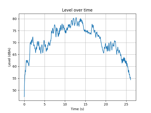
Use the object’s plot() method to plot the level over time (here, level in dBA, for the second signal).

dBA = dBA_time_varying.plot()

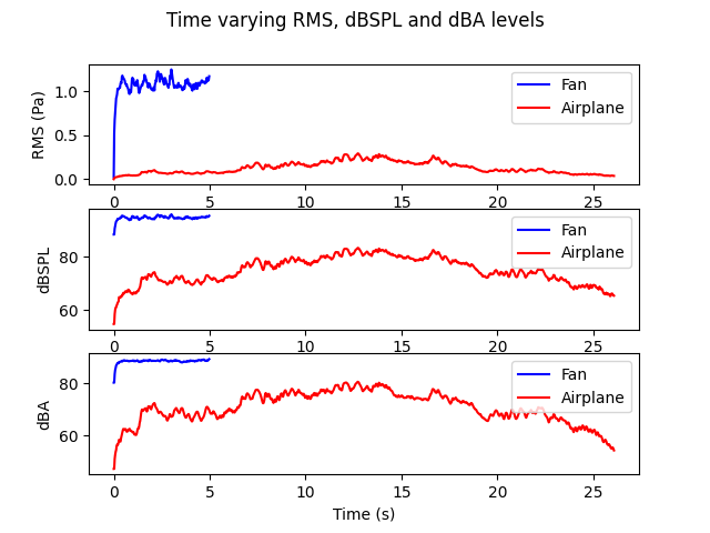
Alternatively, plot the results over time for both signals into three graphs.

fig, axs = plt.subplots(3)
fig.suptitle("Time varying RMS, dBSPL and dBA levels")

axs[0].plot(time[0], rms_levels[0], color="b", label="Fan")
axs[0].plot(time[1], rms_levels[1], color="r", label="Airplane")
axs[0].set_ylabel("RMS (Pa)")
axs[0].legend(loc="upper right")

axs[1].plot(time[0], dBSPL_levels[0], color="b", label="Fan")
axs[1].plot(time[1], dBSPL_levels[1], color="r", label="Airplane")
axs[1].set_ylabel("dBSPL")
axs[1].legend(loc="upper right")

axs[2].plot(time[0], dBA_levels[0], color="b", label="Fan")
axs[2].plot(time[1], dBA_levels[1], color="r", label="Airplane")
axs[2].set_ylabel("dBA")
axs[2].legend(loc="upper right")
axs[2].set_xlabel("Time (s)")

plt.show()