Octave and one-third-octave levels computation

This example shows how to compute 1/3-octave and octave levels, with different methods that are illustrated and compared. Theoretical explanations are also provided at the end of the example, in section Theory, to help understand why these different computation methods exist.

PyAnsys Sound allows computation of octave and one-third-octave levels, whether the input data is:

• a time-domain signal, with classes OctaveLevelsFromSignal and OneThirdOctaveLevelsFromSignal

• a power spectral density (PSD), with classes OctaveLevelsFromPSD and OneThirdOctaveLevelsFromPSD

In the latter case, a specific attribute use_ansi_s1_11_1986 enables you to replicate, when computing band levels from PSD, the effects of the ANSI S1.11-1986 and IEC 61260:1995 band-pass filters used in signal-based classes. This allows meaningful comparisons between levels computed from PSD (for example, from numerical simulations) and levels computed from time-domain signals. See section Comparing octave and one-third-octave levels from signal and from PSD for more details.

Set up analysis

Setting up the analysis consists of loading Ansys libraries, connecting to the DPF server, and downloading the necessary data files.

# Load standard libraries.
import matplotlib.pyplot as plt

# Load Ansys libraries.
from ansys.sound.core import REFERENCE_ACOUSTIC_PRESSURE_IN_AIR
from ansys.sound.core.examples_helpers import download_flute_wav
from ansys.sound.core.server_helpers import connect_to_or_start_server
from ansys.sound.core.signal_utilities import LoadWav
from ansys.sound.core.spectral_processing import PowerSpectralDensity
from ansys.sound.core.standard_levels import (
    OctaveLevelsFromSignal,
    OneThirdOctaveLevelsFromPSD,
    OneThirdOctaveLevelsFromSignal,
)

# Connect to a remote DPF server or start a local DPF server.
my_server, my_license_context = connect_to_or_start_server(use_license_context=True)

# Download the necessary files for this example.
flute_wav_files_path = download_flute_wav()

Octave and one-third-octave levels from signal

Here we show how to compute octave levels using the class OctaveLevelsFromSignal. The same workflow can be replicated for one-third-octave levels using the class OneThirdOctaveLevelsFromSignal.

# Load the time-domain signal from a WAV file.
wav_loader = LoadWav(flute_wav_files_path)
wav_loader.process()
signal_flute = wav_loader.get_output()[0]

# Compute octave levels.
octave_levels = OctaveLevelsFromSignal(
    signal=signal_flute,
    reference_value=REFERENCE_ACOUSTIC_PRESSURE_IN_AIR,
)
octave_levels.process()
band_levels_from_signal, center_frequencies = octave_levels.get_output_as_nparray()

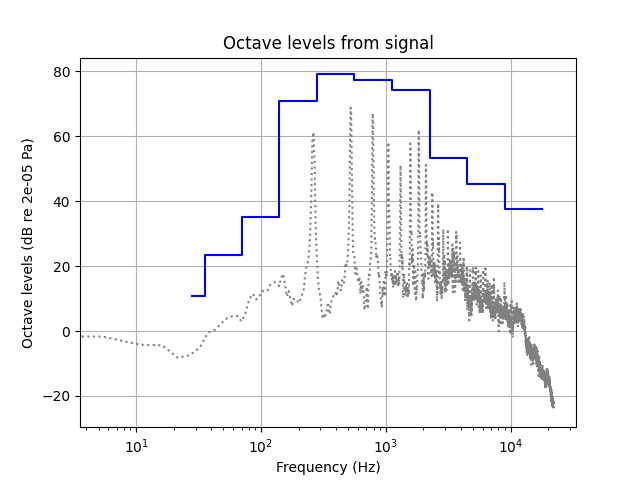
For comparison, let us compute the power spectral density (PSD) from the time-domain signal, and display octave levels and PSD on the same graph.

# Compute the PSD.
psd = PowerSpectralDensity(signal_flute, fft_size=8192, window_length=8192, overlap=0.9)
psd.process()
psd_levels_dB_per_Hz = psd.get_PSD_dB_as_nparray(ref_value=REFERENCE_ACOUSTIC_PRESSURE_IN_AIR)
psd_frequencies = psd.get_frequencies()

# Plot octave levels and PSD on a single graph.
limit_frequencies = (
    [center_frequencies[0] / pow(2, 1 / 6)]
    + [x * pow(2, 1 / 6) for x in center_frequencies[0:-1] for _ in range(2)]
    + [center_frequencies[-1] * pow(2, 1 / 6)]
)
levels_at_limit_frequencies_from_signal = [x for x in band_levels_from_signal for _ in range(2)]

plt.figure()
plt.semilogx(psd_frequencies, psd_levels_dB_per_Hz, label="PSD", color="gray", linestyle=":")
plt.semilogx(
    limit_frequencies,
    levels_at_limit_frequencies_from_signal,
    label="Octave levels from signal",
    color="blue",
    linestyle="-",
)

plt.title("Octave levels from signal")
plt.xlabel("Frequency (Hz)")
plt.ylabel(f"Octave levels (dB re {REFERENCE_ACOUSTIC_PRESSURE_IN_AIR} {signal_flute.unit})")
plt.grid()
plt.show()

Comparing octave and one-third-octave levels from signal and from PSD

Let us now consider a scenario where we wish to compare one-third-octave levels between simulation results - in the form of a PSD - and test data - in the form of a recorded time-domain signal. We consider the case of one-third-octave levels here, but the same can be done for octave levels. For demonstration purposes, we can use the PSD already computed above. As it comes from the same signal, we would then expect the same band levels regardless of the class used, OneThirdOctaveLevelsFromSignal or OneThirdOctaveLevelsFromPSD.

# Compute 1/3-octave levels from the signal.
one_third_octave_levels = OneThirdOctaveLevelsFromSignal(
    signal=signal_flute,
    reference_value=REFERENCE_ACOUSTIC_PRESSURE_IN_AIR,
)
one_third_octave_levels.process()
band_levels_from_signal, center_frequencies = one_third_octave_levels.get_output_as_nparray()

# Compute 1/3-octave levels from the PSD (previously computed from the same signal).
one_third_octave_levels_psd = OneThirdOctaveLevelsFromPSD(
    psd.get_output(),
    reference_value=REFERENCE_ACOUSTIC_PRESSURE_IN_AIR,
)
one_third_octave_levels_psd.process()
band_levels_from_psd = one_third_octave_levels_psd.get_band_levels()

Now, let us compare the two.

# Prepare data for staircase plot of band levels.
limit_frequencies = (
    [center_frequencies[0] / pow(2, 1 / 6)]
    + [x * pow(2, 1 / 6) for x in center_frequencies[0:-1] for _ in range(2)]
    + [center_frequencies[-1] * pow(2, 1 / 6)]
)
levels_at_limit_frequencies_from_signal = [x for x in band_levels_from_signal for _ in range(2)]
levels_at_limit_frequencies_from_psd = [x for x in band_levels_from_psd for _ in range(2)]

# Plot band levels from both data types.
plt.figure()
plt.semilogx(
    limit_frequencies,
    levels_at_limit_frequencies_from_signal,
    label="1/3-octave levels from signal",
    color="red",
    linestyle="-",
)
plt.semilogx(
    limit_frequencies,
    levels_at_limit_frequencies_from_psd,
    label="1/3-octave levels from PSD",
    color="blue",
    linestyle="--",
)
plt.title("1/3-octave levels from signal and from PSD")
plt.xlabel("Frequency (Hz)")
plt.ylabel(f"1/3-octave levels (dB re {REFERENCE_ACOUSTIC_PRESSURE_IN_AIR} {signal_flute.unit})")
plt.xticks(rotation=90)
plt.grid()
plt.legend()
plt.show()

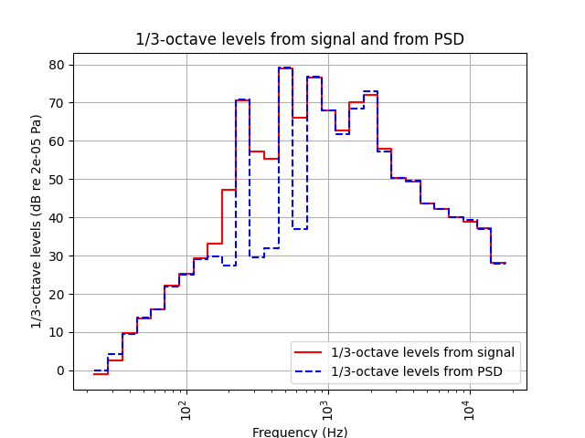
Contrary to our initial assumption, the two methods do not yield identical results, with even very large differences (20-30 dB) in some bands. This discrepancy is due to the neighboring-band leakage effect that is inherent to the filterbank specified in the ANSI S1.11-1986 and IEC 61260:1995 standards, and that the class OneThirdOctaveLevelsFromSignal implements: since the frequency responses of the specified band-pass filters are not perfectly rectangular (due to their finite filter order), each estimated band level is also affected by neighbouring-band frequency contributions. With class OneThirdOctaveLevelsFromPSD, however, the PSD is simply summed up within each band, excluding any contribution from frequencies outside the band. See Theory for more computational details.

Now, let us repeat the PSD-based computation, this time setting the attribute use_ansi_s1_11_1986 to True to replicate the effect of the ANSI S1.11-1986 and IEC 61260:1995 standards’ band-pass filters on the PSD, before computing the band levels.

one_third_octave_levels_psd.use_ansi_s1_11_1986 = True
one_third_octave_levels_psd.process()
band_levels_from_psd = one_third_octave_levels_psd.get_band_levels()

Let us compare the results again.

# Prepare data for staircase plot of band levels.
levels_at_limit_frequencies_from_psd = [x for x in band_levels_from_psd for _ in range(2)]

# Plot against the signal-based levels again.
plt.figure()
plt.semilogx(
    limit_frequencies,
    levels_at_limit_frequencies_from_signal,
    label="1/3-octave levels from signal",
    color="red",
    linestyle="-",
)
plt.semilogx(
    limit_frequencies,
    levels_at_limit_frequencies_from_psd,
    label="1/3-octave levels from PSD (use_ansi_s1_11_1986=True)",
    color="blue",
    linestyle="--",
)
plt.title("1/3-octave levels from signal and from PSD")
plt.xlabel("Frequency (Hz)")
plt.ylabel(f"1/3-octave levels (dB re {REFERENCE_ACOUSTIC_PRESSURE_IN_AIR} {signal_flute.unit})")
plt.grid()
plt.legend()
plt.show()

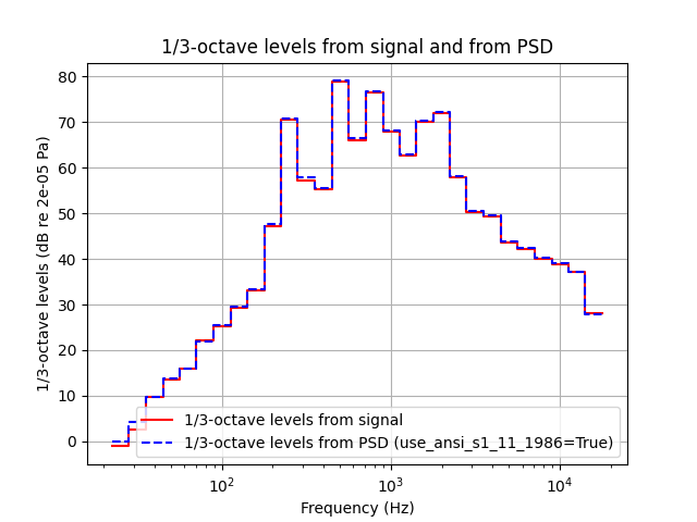
Now, the levels computed from the PSD (with ANSI S1.11-1986 weighting) match those from the signal much more closely.

Takeaways

The previous exemplified scenario emphasizes the importance of selecting the appropriate approach depending on the nature of the input data, and the goal of the analysis:

• For time-domain signals, use signal-based classes to follow the standards, or compute their PSD and then use PSD-based classes to avoid the neighboring-band leakage effect.

• For PSD data, use PSD-based classes, with the use_ansi_s1_11_1986 set to False if you wish to avoid the neighboring-band leakage effect, or True if you wish to approximate standardized results.

• Finally, when working with both signal and PSD data, to ensure comparability of results, either compute PSD from signals and then use PSD-based classes, or use both signal- and PSD-based classes, but make sure to set the use_ansi_s1_11_1986 attribute of PSD-based classes to True.

In any case, keep in mind that following the ANSI S1.11-1986 and IEC 61260:1995 standards (signal-based classes, or PSD-based classes with use_ansi_s1_11_1986 set to True) affects the results with the neighboring-band leakage effect. However, using the PowerSpectralDensity class to compute PSD from signals before using PSD-based classes also affects the results, as the PSD computation parameters have a significant influence on the computed band levels, notably in the narrower, low-frequency bands.

The table below summarizes the different approaches, and their specificities (for the case of octave levels only, but it equally applies for the case of one-third-octave levels).

Input data	Method (classes used)	use_ansi_s1_11_1986	Standard-compliant	Neighboring-band leakage effect	PSD parameters’ effect
Signal	OctaveLevelsFromSignal	N/A	Yes	x
Signal	PowerSpectralDensity OctaveLevelsFromPSD	False	No		x
PSD	OctaveLevelsFromPSD	False	No
PSD	OctaveLevelsFromPSD	True	Yes	x
Signal & PSD	OctaveLevelsFromSignal OctaveLevelsFromPSD	True	Yes	x
Signal & PSD	PowerSpectralDensity OctaveLevelsFromPSD	False	No		x

Theory

This section provides details on the different methods used to compute octave- and one-third-octave-band levels from a time-domain signal and from a power spectral density (PSD).

Octave and one-third-octave levels

Octave and one-third-octave levels are analysis methods to assess how the energy of a signal is distributed across specific frequency bands, defined logarithmically to better match how the frequency scale is perceived by human ears.

An octave is the frequency interval between two frequencies that have a ratio of 2. For example, there is exactly one octave between 50 Hz and 100 Hz, but also between 1000 Hz and 2000 Hz. “Octave bands” are generally understood as a set of 10 predefined, contiguous frequency bands extending over one octave exactly and covering the entire audible frequency range. Notably, each octave band is twice as wide as the previous one, and half as wide as the next one.

One-third-octave bands are a further logarithmic subdivision of each octave band into 3 sub-bands.

The ANSI S1.11-1986 and IEC 61260:1995 standards specify band-pass filters allowing the computation of 29 one-third-octave-band levels from a time-domain signal. Octave-band levels are then derived from one-third-octave levels by summing the computed energy within each set of 3 consecutive one-third-octave bands.

Levels from signal

Band level computation in classes OneThirdOctaveLevelsFromSignal and OctaveLevelsFromSignal follows the ANSI S1.11-1986 and IEC 61260:1995 standards.

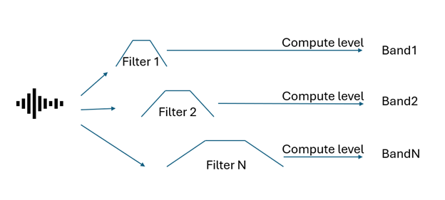
1. The signal is filtered using one-third-octave band-pass filters, resulting in as many band-filtered signals as there are one-third-octaves. Each band-pass filter has a bandwidth of 1/3 of an octave.

2. For each band, the band level is obtained by calculating the overall level of the band-pass-filtered signal.

3. In the case of octave levels, the band levels are then derived by summing the energies obtained for the 3 consecutive one-third-octave bands within each octave band.

The figure below illustrates this process.

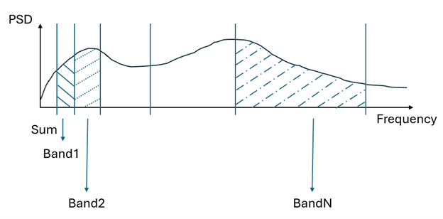
Levels from PSD

Band level computation in classes OneThirdOctaveLevelsFromPSD and OctaveLevelsFromPSD, when attribute use_ansi_s1_11_1986 is set to False (default), simply consists of the integration of the PSD over the frequency range corresponding to a each octave or one-third-octave band.

The figure below illustrates this process.

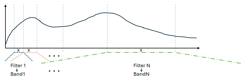
Levels from PSD with ANSI S1.11-1986 weighting

Band level computation in classes OneThirdOctaveLevelsFromPSD and OctaveLevelsFromPSD, when their attribute use_ansi_s1_11_1986 is set to True, precedes the band-wise PSD integration with a PSD weighting according to the frequency responses of the band-pass filters defined in the ANSI S1.11-1986 and IEC61260:1995 standards.

This allows comparing simulation results with measurements in a meaningful way.

1. For each band, the PSD level values are weighted using the frequency response of the band filter defined in the ANSI S1.11-1986 and IEC61260:1995 standards.

2. Each band level is then calculated by integrating the weighted PSD over the whole frequency range.

3. In the case of octave levels, the band levels are again derived by summing the energies obtained for the 3 consecutive one-third-octave bands within each octave band.

The figure below illustrates this process.